Map-driven analysis

Another way to use galpynostatic is to perform an analysis with the map by determining the fundamental parameters involved using another technique (experimental, computational, etc.).

First, we import the libraries that we will use throughout this example.

import galpynostatic as gp
import matplotlib.pyplot as plt
import numpy as np

Compare materials

We can use the map to predict the maximum SOC value of different materials and use it as a figure of merit to compare them.

Suppose we have two different materials (A and B) with the same particle size but different diffusion coefficient and kinetic rate constant properties. We want to know if they are good candidates for a 15 minute load.

d = 0.001

materials = {
    "A": {"dcoeff": 3.7e-9, "k0": 2.03e-7},
    "B": {"dcoeff": 1.17e-11, "k0": 1.14e-6},
}

C_rate = np.array([[4.0]])

We now have all the information we need to describe the system in the model.

spherical = gp.datasets.load_dataset("spherical")
greg = gp.model.GalvanostaticRegressor(d=d)

for m in ("A", "B"):
    # artificial fit
    greg._map = gp.base.MapSpline(spherical)
    greg.dcoeff_ = materials[m]["dcoeff"]
    greg.k0_ = materials[m]["k0"]

    soc_max = greg.predict(C_rate)

    print(f"material {m} has a maximum SOC value of {soc_max[0]:.2f}")

material A has a maximum SOC value of 0.87
material B has a maximum SOC value of 0.02

Here we can see that Material A will retain 87% of its capacity if charged for 15 minutes, while Material B will only retain the 2%. Then material A is a good candidate for a 15 minute charge but material B is not.

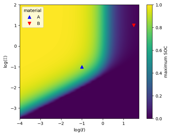
Map visualization

Next, we can see where the materials are located on the map.

fig, ax = plt.subplots()

greg = gp.model.GalvanostaticRegressor(d=d)
greg._map = gp.base.MapSpline(spherical)

ax = greg.plot.render_map(ax=ax)

for m, marker, color in zip(["A", "B"], ["^", "v"], ["blue", "red"]):
    # artificial fit
    greg.dcoeff_ = materials[m]["dcoeff"]
    greg.k0_ = materials[m]["k0"]

    greg.plot.in_render_map(
        C_rate,
        ax=ax,
        marker=marker,
        markersize=7,
        linestyle="",
        color=color,
        label=m,
    )

ax.legend(title="material")
plt.show()

A generalisation of this procedure can be found in the following tutorial.