Benchmarking metrics

In this tutorial we will introduce the galpynostatic.metric module for benchmarking fast charging electrode materials.

First, we will import the libraries that we will use throughout this example.

import galpynostatic as gp
import matplotlib.pyplot as plt
import numpy as np
import pandas as pd

and load the experimental dataset collected and used by Xia et al.

dataset = pd.read_csv("../_static/benchmarking_experimental_data.csv")

Data cleaning

First we will clean the experimental dataset to have it in a proper form for the metric module.

dataset.head()

	Material	particle_size_micro	dcoeff_cm2s
0	Ternary	10	7.8e-11
1	Ternary	8	1.7e-11 to 6.5e-9
2	Ternary	2-5	1e-11 to 3e-11
3	LCO	5-10	1e-11 to 1e-7
4	LCO	NaN	1e-10 to 1.5e-9

We can see that the particle size is given in microns and the range values are separated by a ‘-‘.

dataset["d_mean_micro"] = dataset["particle_size_micro"].str.split("-").apply(
    lambda x: np.mean([float(i) for i in x])
    if isinstance(x, list)
    else np.nan
)

there are also missing values, which we fill in with the mean value of the material group

dataset["d_mean_micro"] = dataset.groupby(
    "Material", group_keys=False
)["d_mean_micro"].apply(lambda x: x.fillna(x.mean()))

In the case of the diffusion coefficient, the range is separated by the characters to and they are spread over a wide range of orders of magnitude, so we use the geometric mean because it is a more appropriate measure than the arithmetic mean, which would be dominated by the larger ones.

from scipy.stats import gmean

dataset["dcoeff_midpoint_cm2s"] = dataset["dcoeff_cm2s"].str.split(" to ").apply(
    lambda x: gmean([float(i) for i in x])
)

Figure of Merit

This metric uses the diffusion coefficient and the particle size to define the characteristic time of diffusion, \(\tau = d^2 / D\). The greater this value, the greater the fast charging capability of the material.

dataset["fom"] = gp.metric.fom(
    1e-4 * dataset["d_mean_micro"], dataset["dcoeff_midpoint_cm2s"]
)

In this case, we generate a chart similar to the one presented by Xia et al.

fig, ax = plt.subplots()

xvalues = np.logspace(-20, -8)
for tau, x, y in zip(
    np.logspace(7, -1, num=5),
    [0.54, 0.72, 0.9, 0.94, 0.94],
    [0.95, 0.95, 0.95, 0.77, 0.56],
):
    ax.plot(xvalues, tau * xvalues, color="tab:gray", linestyle="dashed", linewidth=1)
    exp = np.log10(tau)
    txt = fr"10$^{exp:.0f}$" if exp > 0 else f"{tau:.1f}"
    ax.text(x, y, txt, c="tab:gray", transform=ax.transAxes)

ax.text(0.68, 0.2, r"Less $\tau$ [s]", c="tab:gray", transform=ax.transAxes)
ax.text(0.68, 0.15, r"Xia et al. faster", c="tab:gray", transform=ax.transAxes)
ax.text(0.68, 0.1, r"charging", c="tab:gray", transform=ax.transAxes)

marker, color = {}, {}
for material, m, c in zip(
    ("LCO", "LMO", "LTO", "LFP", "Ternary", "Graphite"),
    ("s", "o", "D", "^", "v", "<"),
    (None, "red", "pink", "blue", "green", "orange")
):
    marker[material] = m
    color[material] = f"tab:{c}" if c is not None else "k"

for m, d, dcoeff, tau in dataset[
    ["Material", "d_mean_micro", "dcoeff_midpoint_cm2s", "fom"]
].values:
    ax.scatter(1e-4 * dcoeff, (1e-6 * d)**2, marker=marker[m], color=color[m], label=m)

ax.set_xlim((7e-20, 1e-8))
ax.set_xlabel(r"Diffusion coefficient $D$ [m$^2$/s]")
ax.set_xscale("log")

ax.set_ylim((1e-15, 1e-6))
ax.set_ylabel(r"Square of geometric size $d^2$ [$m^2$]")
ax.set_yscale("log")

handles, labels = ax.get_legend_handles_labels()
unique_labels, unique_handles = {}, []
for label, handle in zip(labels, handles):
    if label not in unique_labels:
        unique_labels[label] = handle
        unique_handles.append(handle)

ax.legend(unique_handles, unique_labels.keys())

plt.show()

BMXFC

This universal metric for Benchmarking battery electrode Materials for eXtreme Fast-Charging (BMXFC) is defined as the State-of-Charge reached when a material is charged for 15 minutes under constant current conditions. It gives possible values between 0 and 1 and it is directly the percentage of charge retained.

dataset["full_bmxfc"] = [
    gp.metric.bmxfc(
        {"d": 1.0e-4 * d, "dcoeff_": dcoeff, "k0_": 5.0e-8}, full_output=True
    )
    for m, d, dcoeff, tau in dataset[
        ["Material", "d_mean_micro", "dcoeff_midpoint_cm2s", "fom"]
    ].values
]

This full_output returns not only the bmxfc value, but also if it meets the fast charging criteria (\(\text{BMXFC} \geq 0.8\)), and a GalvanostaticRegressor object to plot each material in the map and make predictions.

fig, ax = plt.subplots()
dataset["full_bmxfc"][0]["greg"].plot.render_map(ax=ax, clb_label="BMXFC")

for m, material in dataset[["Material", "full_bmxfc"]].values:
    ax = material["greg"].plot.in_render_map(
        np.array([[4.0]]), ax=ax, marker=marker[m], color=color[m], label=m
    )

ax.set_xlim((-4, 1.75))
ax.set_ylim((-3.5, 2))

ax.legend(unique_handles, unique_labels.keys(), ncol=6, loc=(-0.25, 1.05))

plt.show()

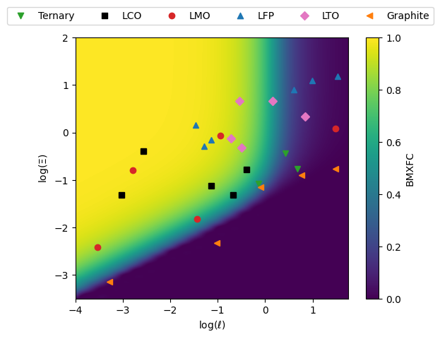
We can see here which materials are classified as fast charging ones (yellow zone) and which are not (purple zone).