Heuristic model

We will fit our heuristic model by using experimental data from the Lei et al. paper for the LFP system.

First, we import the libraries that we will use throughout this example:

import galpynostatic as gp
import matplotlib.pyplot as plt
import numpy as np
import pandas as pd

Data visualization

We define a numpy array with the C-rates that were used to perform the measurements in the experiment.

C_rates = np.array([0.2, 0.5, 1, 2, 5, 10])

For each one of these C-rates we have a galvanostatic profile as a csv file, which we read with pandas and store in a list for further preprocessing.

gprofiles = [pd.read_csv(f"../_static/{c_rate}C.csv") for c_rate in C_rates]
gprofiles[0].keys()

Index(['capacity', 'voltage'], dtype='object')

we have a pd.DataFrame for each curve with a capacity and a voltage column. We also define from their work the equilibrium potential and our choice for the cut-off potential (which is that of the distributed map datasets).

eq_pot, vcut = 3.45, 0.15

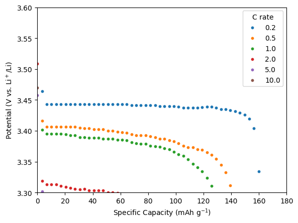
We plot the curves to visualize them in the region of interest:

fig, ax = plt.subplots()

for c_rate, df in zip(C_rates, gprofiles):
    ax.scatter(df.capacity, df.voltage, s=10, label=f"{c_rate}")

ax.set_xlim((0, 180))
ax.set_ylim((eq_pot - vcut, eq_pot + vcut))
ax.set_xlabel(r"Specific Capacity (mAh g$^{-1}$)")
ax.set_ylabel(r"Potential (V vs. Li$^+$/Li)")
ax.legend(title="C rate")
plt.show()

Data preprocessing

In the physics-based heuristic model presented here, we are not interested in the complete behavior of the profile, but focus our analysis on the points where each curve intersects at a cut-off potential below the equilibrium potential. To obtain these values we can use the galpynostatic.preprocessing module.

gdc = gp.preprocessing.GetDischargeCapacities(eq_pot=eq_pot, vcut=vcut)
dc = gdc.fit_transform(gprofiles)
dc

array([160.27912017, 141.21537819, 128.30040942,  55.62272794,
         3.53156547,   1.62308932])

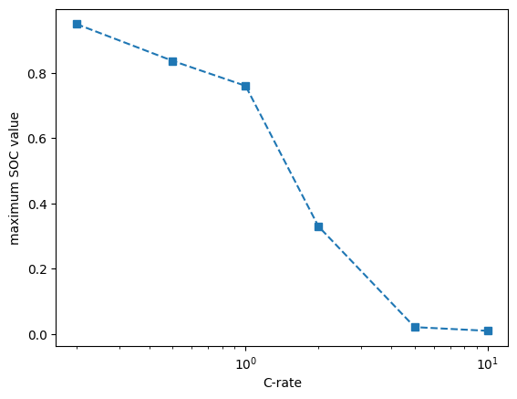
We need to normalize these currents by a maximum value that we define (here we use the maximum value of the capacity for the lowest C-rate reported in the paper, which is 168.9 mAh g\(^{-1}\)) to obtain the maximum SOC value between 0 and 1, which will be the target values for the fitting of our model.

soc = dc / 168.9

Model fitting

First, the data is displayed in the form it will be used by the model.

fig, ax = plt.subplots()

plt.plot(C_rates, soc, marker="s", ls="--")

plt.xlabel("C-rate")
plt.ylabel("maximum SOC value")
plt.xscale("log")
plt.show()

and reshape the C-rate values according to the scikit-learn convention.

C_rates = C_rates.reshape(-1, 1)

In the paper it is mentioned that the particle sizes are distributed between 200-500 nm, we take the center and give it in cm, which is the required unit for this parameter.

d = 3.5e-5

We use the default surface data for spherical geometry with a cut-off potential of 150 mV and the corresponding default z-value of 3.

greg = gp.model.GalvanostaticRegressor(d=d)
greg.fit(C_rates, soc)

GalvanostaticRegressor(d=3.5e-05,
                       dataset=         l   xi     xmax
0    -4.00  2.0  0.99706
1    -4.00  1.9  0.99706
2    -4.00  1.8  0.99705
3    -4.00  1.7  0.99705
4    -4.00  1.6  0.99705
...    ...  ...      ...
1339  1.75 -3.1  0.00000
1340  1.75 -3.2  0.00000
1341  1.75 -3.3  0.00000
1342  1.75 -3.4  0.00000
1343  1.75 -3.5  0.00000

[1344 rows x 3 columns])

In a Jupyter environment, please rerun this cell to show the HTML representation or trust the notebook.
On GitHub, the HTML representation is unable to render, please try loading this page with nbviewer.org.

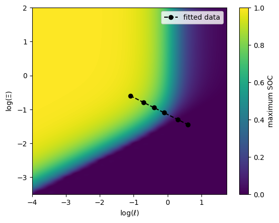
Two types of plots are available, one to visualize the region of the map where the experimental data are located after the fitting

greg.plot.in_render_map(C_rates)
plt.legend()
plt.show()

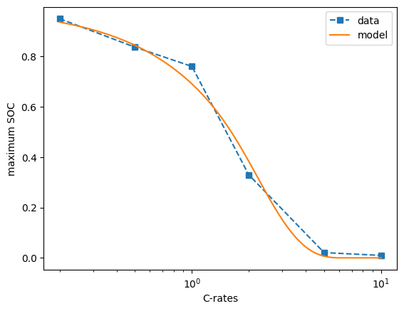
and another to visualize the predicted versus experimental values in the same format as used for the fitting.

greg.plot.versus_data(C_rates, soc)
plt.legend()
plt.show()

Predictions

We can obtain fundamental parameters of the system by accessing attributes of the GalvanostaticRegressor model, such as the diffusion coefficient (with its uncertainty)

print(f"{greg.dcoeff_:.2e} +/- {greg.dcoeff_err_:.0e} cm^2/s")

2.85e-13 +/- 1e-14 cm^2/s

which in this case is in good agreement with the three values of 1.04e-12, 1.74e-13 and 8.22e-13 (EIS measurements) reported in their paper. In addition, we can obtain the kinetic rate constant

print(f"{greg.k0_:.2e} +/- {greg.k0_err_:.0e} cm/s")

1.00e-09 +/- 3e-11 cm/s

which is also in good agreement with the experimental value of 1.23e-9, calculated using the Butler-Volmer equation with the reported exchange current density value.

Finally, there is a fast-charging criteria, proposed by the United States Advanced Battery Consortium (USABC), which aims for an extremely fast-charging of 80% SOC (State-of-Charge) in 15 minutes. This corresponds to a maximum SOC value of 0.8 and a C-rate of 4C. A prediction of the particle size needed to meet this criterion can be quickly made using the optimal_particle_size function in the galpynostatic.make_prediction module (which has the default values of the criterion defined).

d_new, d_new_err = gp.make_prediction.optimal_particle_size(greg, d0=1e-5)
print(f"{d_new:.3f} +/- {d_new_err:.3f} micrometers")

0.084 +/- 0.002 micrometers

This predicted value can be compared to the original value (d)

1e4 * d

0.35

where it can be seen that our model predicts that the system should be improved by reducing the particle size by about an order of magnitude.